In this post, I explain the meaning of some frequently used geographies in the UK, which I use extensively in other posts of this blog. Additionally, I explain the basics of how to plot them in Python using GeoPandas, and data sources for useful files with UK geographies.
Official UK Geographies
When working with official geographies, we will usually find there are hierarchies, where a geography is consecutively subdivided into smaller levels. In the UK, there are two common hierarchies: administrative and statistical. An excellent source that explains both in detail can be found on the London Borough of Tower Hamlets site. For a short explanation, see below:
Statistical hierarchy
It was created mainly for census purposes. The geographies in this hierarchy are not commonly known to the public, they are more intended for analysis of census information. Usually, each unit is represented just by a code rather than by a name.
The smallest geography in this hierarchy is the Output Area (OA). It was sought that each one contains a similar number of inhabitants and was homogeneous in terms of different census variables such as home tenure, etc.
The next higher level is that of the Lower Super Output Areas (LSOAs), which are nothing more than groups of OAs. In my opinion, LSOAs are an ideal size to analyse geographic data in detail.
The upper level is made up of Middle Layer Super Output Areas (MSOAs), which are groups of LSOAs.
Administrative Hierarchy
In this hierarchy, the geographies were not created for census purposes, and therefore do not comply with any rules related to their population or dwelling types. Its limits have mixed origins, from historical to given by administrative practicality (electoral administration, etc).
Wards, one of the smallest administrative units, are defined as groups of LSOAs, so although they are administrative geographies, it is also easy to aggregate statistical/census data by Ward. Then we have Local Authorities, which are sets of Wards. In London, they are also known as Boroughs. This hierarchy is much more familiar to the public. It is much more common for people to know which Ward they live in, and definitely which Borough they live in.
Wards are the closest thing to the concept of neighbourhood. However, the official limits of different Wards do not always coincide with the limits of the neighbourhoods that the public is familiar with.
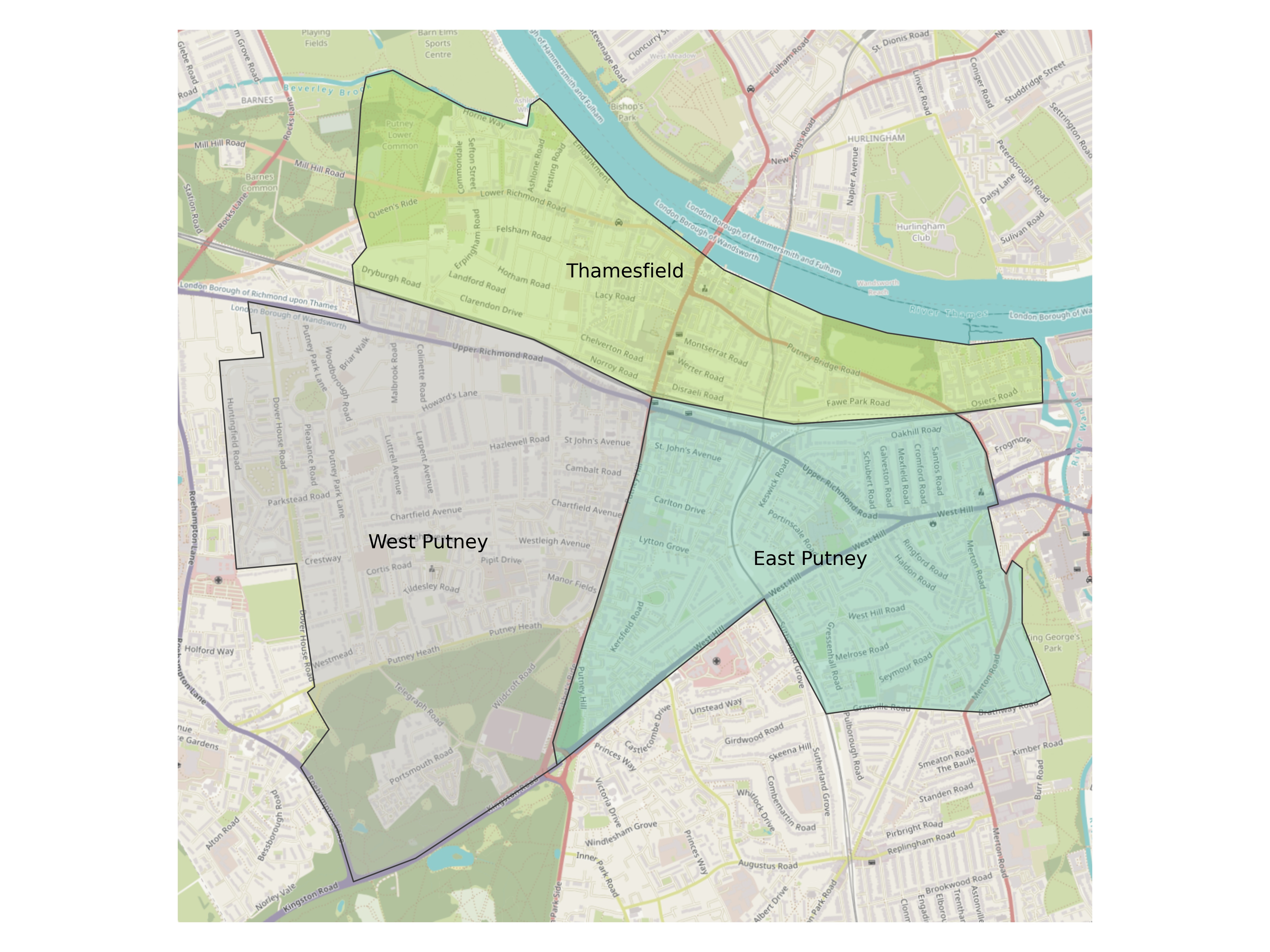
For example, the area known as Putney, in South West London, falls within three different wards:
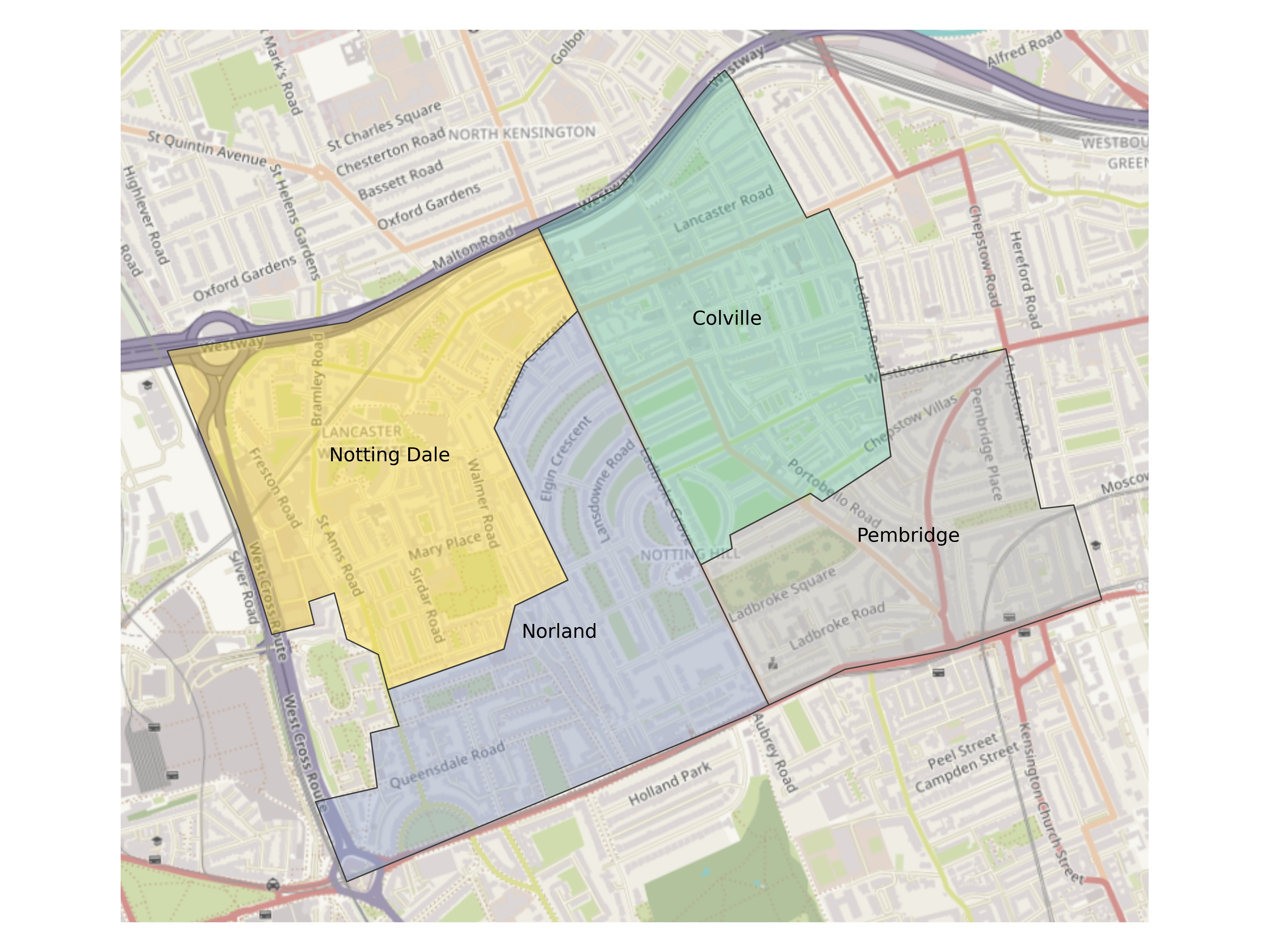
And the famous Notting Hill neighbourhood, not only is not represented by a single Ward but also doesn’t actually give its name to any of the wards falling within its commonly acknowledged borders.
As a final example, the image below presents a comparative view featuring Westminster Borough, the distinctive ward of St James’s (home to the Palace of Westminster), and the Lower Layer Super Output Areas (LSOAs) that this ward comprises.
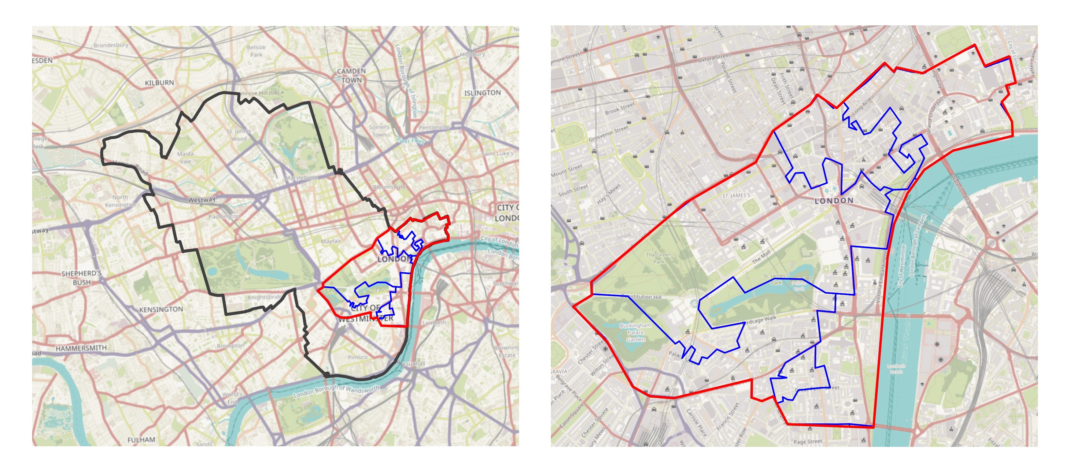 Westminster Borough (grey), St James’s Ward (red), LSOAs (blue)
The next section will show the Python code to produce that last plot.
Plotting with GeoPandas
To plot with Geopandas, we need to have the data in a GeoDataFrame. This structure works like a DataFrame, but it has also a column with the shape (geometry) associated with each row. It also contains an indication of which coordinate reference system (CRS) it uses.
There are multiple ways to obtain a GeoDataFrame, and possibly the easiest is by importing a file that already has the geometries and their metadata. An example of such a file is a shapefiles (files of .shp extension). Various sources, including government sources, offer downloadable shapefiles for ready use.
In the UK, the Office for National Statistics has an Open Geography Portal with plenty of resources, including shapefiles. Available data includes LSOAs, Wards, Post Codes, Parishes, and much more. For example, from these links, you can download shapefiles for:
Once downloaded to our local drive, we can import a shapefile into a GeoDataFrame with:
import geopandas as gpd
shp_lsoa = gpd.read_file(‘London LSOA 2021.shp')
Plotting a GeoDataFrame is straightforward using the method .plot(), which in the case of polygons, will plot filled shapes:
shp_lsoa.plot()
Or if we only want to plot the boundaries instead of filled polygons, we can do it with:
shp_lsoa.boundary.plot()
Optionally, adding a base map to our plot can be done with the package contextily.
contextily.add_basemap()
Below, a full example of how to generate the side-by-side plots of Westimnster Borough, St James’s Ward and its LSOAs that was shown in the previous section.
import matplotlib.pyplot as plt
import geopandas as gpd
import contextily as cx

# import shapefiles
shp_lsoa = gpd.read_file('London LSOAs.shp')
shp_borough = gpd.read_file('London_Boroughs.shp')
shp_ward = gpd.read_file('London Wards.shp')

# plotting function
def plot_borough_ward_lsoa(target_borough, target_ward):

    fig, ax = plt.subplots(1,2, figsize=(5, 2.5))
    plt.subplots_adjust(wspace=0.05)

    # Borough Plot
    # set map limits around target Borough
    shp_borough.query("NAME== @target_borough").\
        buffer(1000).\
        boundary.plot(ax = ax[0], alpha=0)
    # add basemap
    cx.add_basemap(ax = ax[0], crs = shp_borough.crs, alpha=0.9, attribution = False)
    # plot borough
    shp_borough.query("NAME== @target_borough").\
        boundary.plot(ax = ax[0], color='#404040', linewidth = 1)
    # plot LSOAs overlapping with target Ward
    shp_ward.query("WD22NM == @target_ward").\
        overlay(shp_lsoa, how ='identity').\
        boundary.plot(ax = ax[0], color = 'blue', linewidth = 0.5)
    # plot Ward boundary
    shp_ward.query("WD22NM == @target_ward").\
        boundary.plot(ax = ax[0], color = 'red', linewidth = 0.8)
    # remove axis
    ax[0].set_axis_off()

    # Ward and LSOA Plot
    # set map limits around target Ward
    shp_ward.query("WD22NM == @target_ward").\
        boundary.plot(ax = ax[1], alpha=0)
    # add basemap
    cx.add_basemap(ax = ax[1], crs = shp_ward.crs, alpha=0.9, attribution = False)
    # plot LSOAs overlapping with target Ward
    shp_ward.query("WD22NM == @target_ward").\
        overlay(shp_lsoa, how ='identity').\
        boundary.plot(ax = ax[1], color = 'blue', linewidth = 0.5)
    # plot Ward boundary
    shp_ward.query("WD22NM == @target_ward").\
        boundary.plot(ax = ax[1], color = 'red', linewidth = 0.8)
    # remove axis
    ax[1].set_axis_off()

    return fig, ax

# plot target borough and wards
fig, ax = plot_borough_ward_lsoa(target_borough = 'Westminster', target_ward = "St James's")
plt.show()
In subsequent posts, I will use these geographies, as well as GeoPandas plotting capabilities, to explore geographical data in many interesting ways. Watch this space!